Predicting Sales Opportunities
General Assembly Capstone Project
by Daryl Cheong

Introduction
Sales is one of the essential components of any business. It is the act of selling goods or services to an interested party, in exchange for money. It is the primary process for a business to generate revenue, which explains why it is so vital for any organisation. Without sales, a business will not have the resources necessary to grow or even survive.
Due to its importance, this project will examine the sales process of an organisation and seek to achieve the following goals:-
Goal 1 - Predict the value of sales opportunity (‘Amount’ column) using regression models
Goal 2 - Predict the outcome of sales opportunity (‘Result’ column) using classification models
Table of Contents
Part 1 Pre-Processing
1.1 - Data Overview
1.2 - Data Cleaning
1.3 - Exploratory Data Analysis
1.4 - Feature Engineering
Part 2 Predict Opportunity Amount
2.1 - Feature Selection
2.2 - Prepare training/testing data
2.3 - Model Generation
2.4 - Model Results Evaluation
2.5 - Model Selection
Part 3 Predict Opportunity Outcome
3.1 - Prepare training/testing data
3.2 - Data Imbalance
3.3 - Model Generation
3.4 - Model Results Evaluation
3.5 - Model Selection
Conclusion
Part 1 Pre-Processing
1.1 - Data Overview
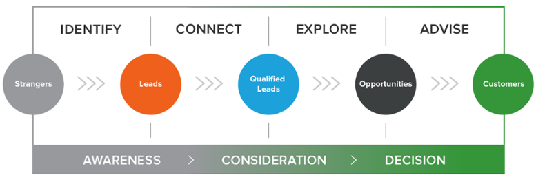
In this project, we will be looking at the sales database for an automotive supplies wholesaler. This is a sample dataset provided by IBM Watson Analytics. The goal of the sales process is to identify and communicate with potential leads, and explore opportunities to convert them into customers. For this project, the database contains records of every sales opportunity with information about the client, product, and process status which focuses on 3 key stages:-
- Identified/Qualifying
- Qualified/Validating
- Validated/Gaining Agreement
This dataset consists of 78,025 rows and 19 columns (9 numerical, 10 categorical). The columns include the following:-
- Amount - Estimated total revenue of opportunities in USD. (Goal 1)
- Result - Outcome of opportunity. (Goal 2)
- Id - A uniquely generated number assigned to the opportunity.
- Supplies - Category for each supplies group.
- Supplies_Sub - Sub group of each supplies group.
- Region - Name of the region.
- Market - The opportunities’ route to market.
- Client_Revenue - Client size based on annual revenue.
- Client_Employee - Client size by number of employees.
- Client_Past - Revenue identified from this client in the past two years.
- Competitor - An indicator if a competitor has been identified.
- Size - Categorical grouping of the opportunity amount.
- Elapsed_Days - The number of days between the change in sales stages. Each change resets the counter.
- Stage_Change - The number of times an opportunity changes sales stage. Includes backward and forward changes.
- Total_Days - Total days spent in Sales Stages from Identified/Validating to Gained Agreement/Closing.
- Total_Siebel - Total days spent in Siebel Stages from Identified/Validating to Qualified/Gaining Agreement.
- Ratio_Identify - Ratio of total days spent in the Identified/Validating stage over total days in sales process.
- Ratio_Validate - Ratio of total days spent in the Validated/Qualifying stage over total days in sales process.
- Ratio_Qualify - Ratio of total days spent in Qualified/Gaining Agreement stage over total days in sales process.
1.2 - Data Cleaning
Before proceeding, it is necessary to conduct checks to evaluate the integrity of the dataset. Incorrect and incomplete data will affect the results of our models, so these issues will need to be identified and addressed first.
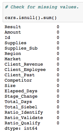
Missing values is a common problem faced in data science. Fortunately, our dataset is complete without any missing values.
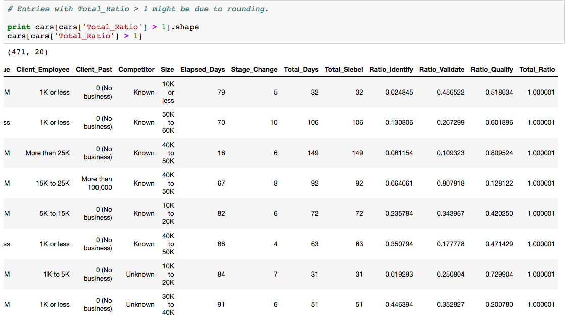
Next, a check will be conducted on the 3 ratio columns (Ratio_Identify, Ratio_Validate, Ratio_Qualify) to ensure that the total value does not exceed 1. A new column Total_Ratio will be created that sums up the values of these 3 columns.
The results of the new Total_Ratio column shows that there are 471 records with a total ratio that exceeds the total of 1. Upon closer inspection, the exceeded amount for each of these records is very minor and it is safe to assume that this is possibly due to the rounding in the 3 ratio columns and thus these records will remain as is.
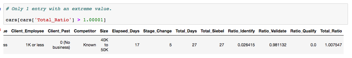
However, there is a single record that has an extreme value of 1.007547. This record will therefore be removed.
The string values for the categorical columns will also be cleaned up to ensure a consistent format.
cars['Client_Employee'].replace(['1K or less', 'More than 25K', '5K to 15K', '1K to 5K', '15K to 25K'],
                                ['Below_1K', 'Above_25K', '5K_to_15K', '1K_to_5K', '15K_to_25K'],
                                inplace=True)
Lastly, the Id and Total_Ratio columns will be dropped since they are no longer necessary.
1.3 - Exploratory Data Analysis
With the data cleaned, we can now carry out EDA and perform an in-depth analysis of the data.
Lets start by examining the correlation between the numerical columns through the construction of a heatmap.
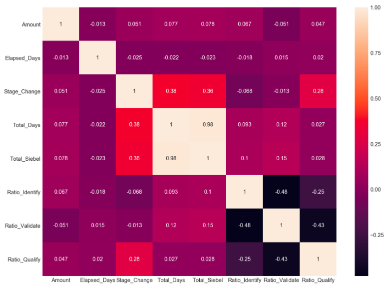
The heatmap above immediately higlights an almost perfect correlation between the Total_Days and Total_Siebel columns. This will have a negative impact on our models, therefore the Total_Siebal column will be dropped. The other numerical columns have a low to moderate correlation value, which are acceptable and no additional measures will be required.
Next, we will analyse the distribution of our features by plotting various graphs.
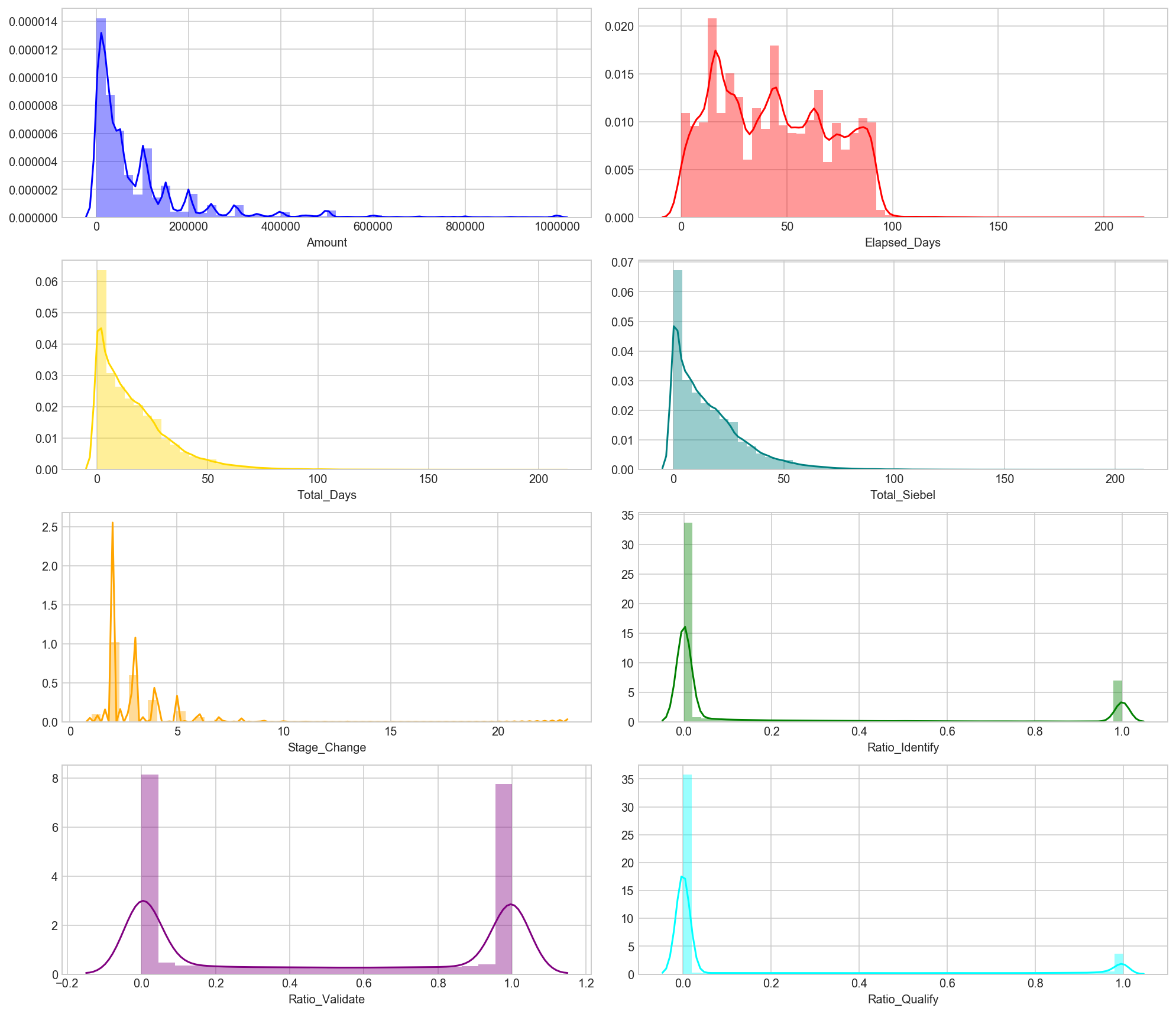
We will use histograms to represent data in the numerical columns. Majority of the graphs show a positively skewed distribution, with very few data points located on the right side. The 3 ratio columns represent data points that are located at both extreme ends of the scale and a minimal number in the middle.
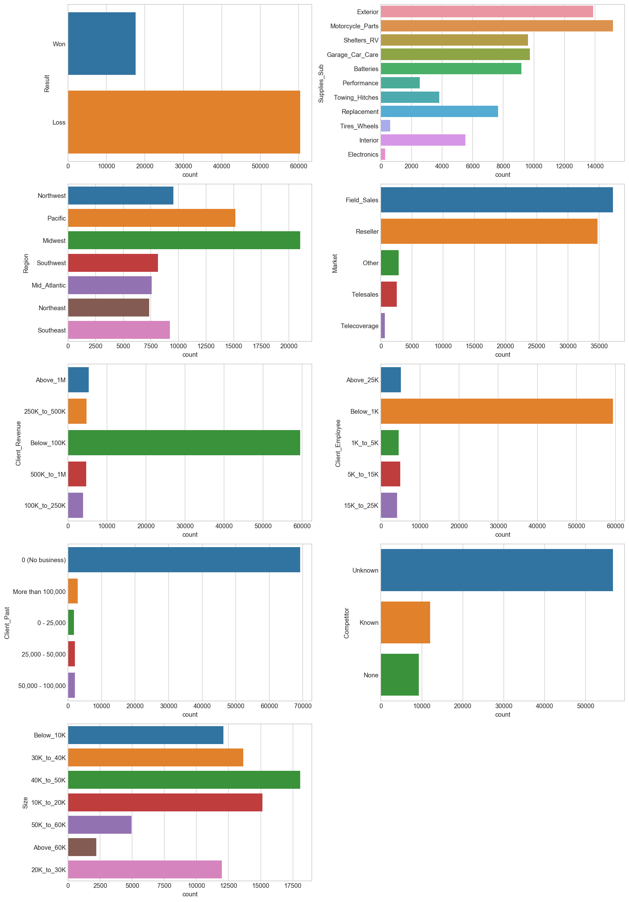
With regards to the categorical columns, bar graphs illustrate the distribution across the different classes. We can see a decent spread across all classes for the Supplies_Sub, Region and Size columns. However, the other features have a strong class imbalance distribution, with a single dominant class. Even our target feature Result has an imbalance where the majority class is about three times larger than the minority class. Class imbalance can have a negative impact on machine learning algorithms, and may result in predictive models that are biased and inaccurate.
1.4 - Feature Engineering
The next stage of pre-processing requires some changes to be made to the current features. The first step involves converting the values in our target column Result into binary values.
cars['Result'] = cars['Result'].map(lambda x: 0 if x == 'Loss' else 1)
The classes in the Client_Past columns are also changed. The data is grouped into 2 classes to identify if the opportunity is from a new client or existing client, rather than separating into 5 classes.
cars['Client_Past'] = cars['Client_Past'].map(lambda x: 0 if x == '0 (No business)' else 1)
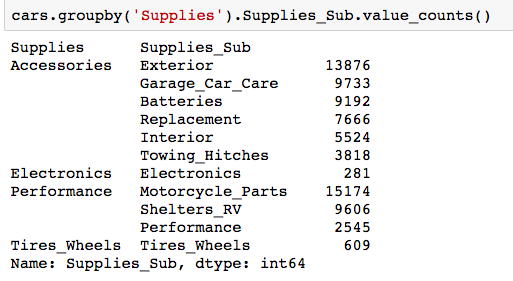
Comparing the Supplies and Supplies_Sub columns, we can see that Supplies_Sub actually is more detailed and provides a clearer picture as compared to Supplies. Therefore, the Supplies column will be dropped.
The Total_Siebel column was previously shown to be highly correlated to the Total_Days column, so that too will be removed.
Due to the number of categorical features in our dataset, we will create 38 new dummy variables to replace the original categorical columns. This new set of dummy variables is then concatenated with the original dataset to create a new dataset to be used our predictions.
cat_dummy = pd.get_dummies(cars2[cat_columns], drop_first=True)
cars2.drop(cat_columns, axis=1, inplace=True)
cars2 = pd.concat([cars2, cat_dummy], axis=1)
With pre-processing completed, we are now ready to commence building our predictive models.
Part 2 Predict Opportunity Amount
All businesses are interested in knowing how much revenue they can make for each transaction, therefore the ability to predict the value of a sales opportunity would be very insightful. In this section, the objective will be to predict the values in the Amount column and through the use of Regression algorithms. But first, we will need to take additional steps to prepare our data for model generation.

2.1 - Feature Selection
We will begin by performing feature selection by using the .summary() command from statsmodels python package to analyse the p-values of each feature. Any features with a p-value or 0.05 and higher will be deemed insignificant and thus dropped.
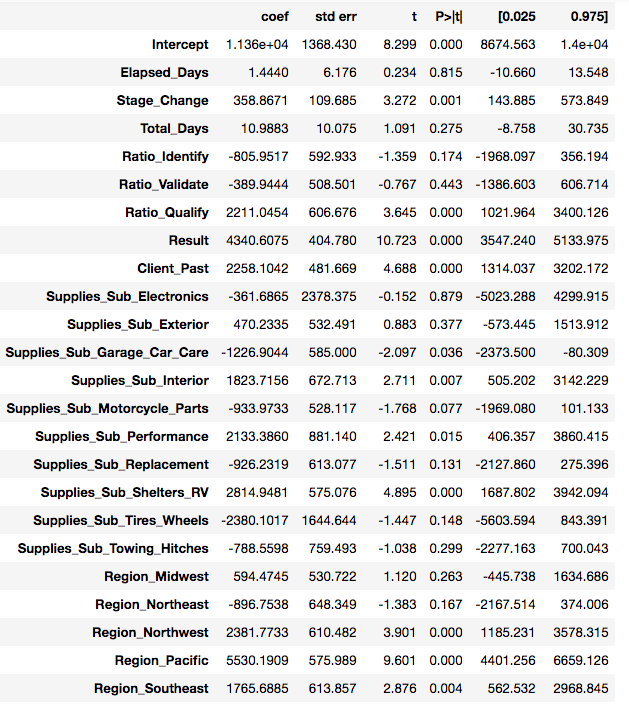
These are the features that were dropped.
cars2.drop(['Ratio_Identify', 'Supplies_Sub_Electronics', 'Supplies_Sub_Garage_Car_Care', 'Market_Other',
            'Client_Revenue_500K_to_1M', 'Client_Revenue_250K_to_500K', 'Supplies_Sub_Towing_Hitches',
            'Client_Revenue_Above_1M', 'Client_Revenue_Below_100K', 'Client_Employee_1K_to_5K',
            'Client_Employee_5K_to_15K', 'Client_Employee_Below_1K', 'Client_Employee_Above_25K',
            'Supplies_Sub_Tires_Wheels', 'Region_Midwest', 'Elapsed_Days', 'Supplies_Sub_Replacement',
            'Supplies_Sub_Motorcycle_Parts', 'Ratio_Validate', 'Total_Days'], axis=1, inplace=True)
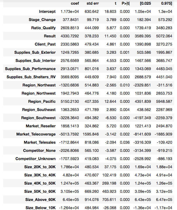
Using this method, 20 out of 44 features were removed. The selected features are shown below.
2.2 - Prepare training/testing data
To prepare our data, we will use the holdout method to split our dataset. We will use training set that comprises of 70% of the data to train our models, and a testing set of 30% to assess their predictions. 5-fold cross validation will also be applied to the training set for all models.
X_train, X_test, y_train, y_test = train_test_split(X, y, train_size=0.7, random_state=100)
2.3 - Model Generation
Model construction can begin by using the new prepared datasets.
5 different regression algorithms will used to create the models:
- Linear Regression
- Lasso Regression
- Ridge Regression
- SGD Regression
- Random Forest Regression
The diagram below is an example of the code used to build the Lasso Regression model.
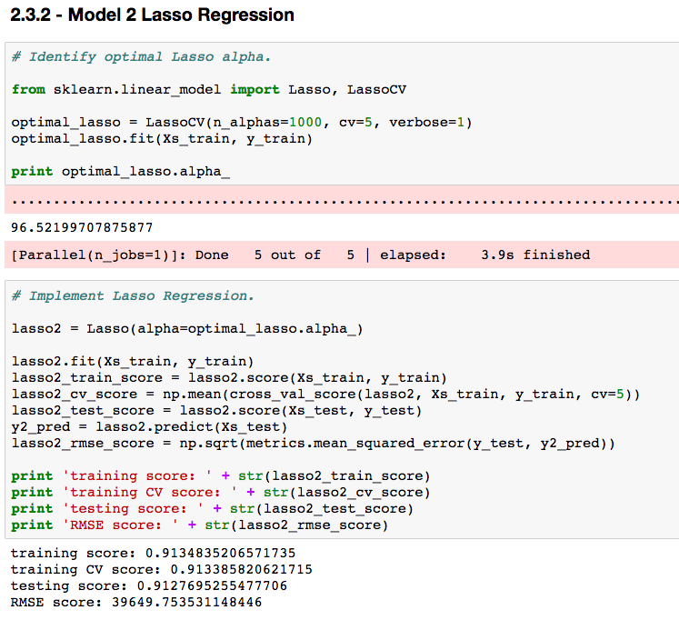
The results for each of the 5 models will be collected and evaluated, before selecting the model that best predicts the opportunity amount.
2.4 - Model Results Evaluation
With the models completed, we can now compile all the results into a new pandas dataframe, making it easier to compare the results. Graphical representations will also be generated to help visualise the output.
Model performance will be judged based on 2 key criterias:-
- R^2 score (training, cross validation, testing)
- Root Mean Squared Error score (RMSE)
We will also take a look at the feature rankings for the models.
When conducting evaluation, we are looking for a model with a high R^2 score and low RMSE score. The R^2 score would indicate the goodness of fit of a set of predictions on the actual values, RMSE indicates the magnitude of error between the predicted and actual value in terms of the output value.
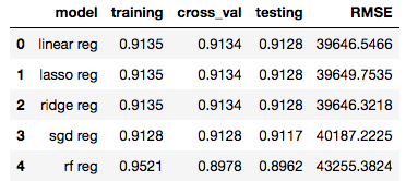
Looking at the compiled results, we see that Linear, Lasso and Ridge Regression achieved the highest R^2 scores, and the results were identical. Even their RMSE scores were almost exact. On the other hand, the Random Forest Regression model performed the worst with the lowest R^2 score and highest RMSE score.
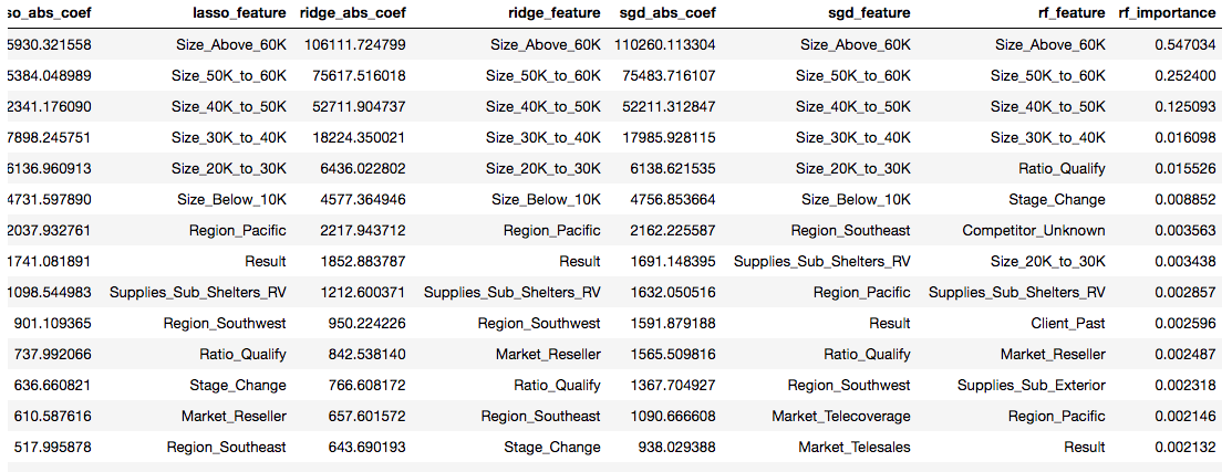
In terms of feature ranking, all 5 models share the same features that occupy the top 4 ranks, which are Size_above_60K, Size_50K_to_60K, Size_40K_to_50K and Size_30K_to_40K. After that, feature rankings begin to differentiate between models. These top 4 features also have very similar coefficient values, with the exception of the Random Forest Regression model which uses a different weights scale. The coefficient values show us how large of an impact a particular feature has on the overall opportunity amount.
2.5 - Model Selection
As mentioned earlier, the ideal model is judged according to their R^2 and RMSE scores. As Linear Regression, Lasso Regression and Ridge Regression had the highest R^2 testing score and their values are identical, we will then compare the RMSE score between these 3 models. Based on our evaluation of the results above, we can conclude that the Ridge Regression model is the best choice with the lowest RMSE score of 39646.3218.
Part 3 Predict Opportunity Outcome

In part 3 of this project, we will now create classification models to predict the sales opportunity outcome (Result column). The ability to predict the outcome enables a business to identify influencing factors and also better utilize their resources.
Previously in our pre-processing stage, we converted the values in the Result column into binary numbers. The value 1 represents the opportunities that were won, while the value 0 signifies the opportunities that were lost. Hence, our goal will be to accurately predict the highest number of 1s.
3.1 - Prepare training/testing data
For this prediction, we will also be using the holdout method to create the training and testing datasets, and incorporating 5-fold cross-validation into the models.
The next step incorporates the SelectFromModel function from sklearn to perform feature selection, and apply the RandomForestClassifier inside the function as an estimator to identify the feature importance.
from sklearn.feature_selection import SelectFromModel
from sklearn.ensemble import RandomForestClassifier
select = SelectFromModel(RandomForestClassifier())
select.fit(Xs_train, y_train)
Xs_train = select.transform(Xs_train)
Xs_test = select.transform(Xs_test)
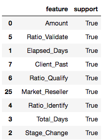
feature_support = pd.DataFrame({'feature': X_train.columns, 'support': select.get_support()})
feature_support.sort_values('support', inplace=True, ascending=False)
feature_support.head(10)
The results show that out of the 44 features in our dataset, only 9 were selected. This means that these 9 features had the biggest influence in prediction the opportunity outcome.
3.2 - Data Imbalance
As previously shown in our distribution plots under the EDA section, there is an imbalance in our target column whereby the majority class 0 has a total count of more than 3 times when compared to the minority class 1. To solve the problem of class imbalance, we will utilize 2 different techniques from the python package imblearn to resample the data in our training set.
RandomOverSampler - randomly oversample the minority class (1) with replacement.
from imblearn.over_sampling import RandomOverSampler
ros = RandomOverSampler(random_state=100)
Xs_train_ros, y_train_ros = ros.fit_sample(Xs_train, y_train)
RandomUnderSampler - randomly undersample the majority class (0) with replacement.
from imblearn.under_sampling import RandomUnderSampler
rus = RandomUnderSampler(random_state=100)
Xs_train_rus, y_train_rus = rus.fit_sample(Xs_train, y_train)
Oversampling will increase the number of minority class from 12401 to 42215, while undersampling will reduce the number of majority class from 42215 to 12401. The end result after resampling is 3 different training sets (default, oversample, undersample).
3.3 - Model Generation
Now that we have our training and testing datasets, we can begin to generate our models.
3 different classification algorithms will used to create the models:
- Logistic Regression
- Random Forest
- K-Nearest Neighbors
3 versions of each algorithm will also be created, with each version tackling a different dataset (default, oversample, undersample). In the end, we will have 9 models to compare. The results for each of the 9 models will be collected and evaluated, before selecting the model that best predicts the opportunity result.
3.4 - Model Results Evaluation
With the models completed, we can now compile all the results into a new pandas dataframe, making it easier to compare the results. Graphical representations will also be generated to help visualise the output.
An example of the output results for the Logistic Regression (default) model is shown below.
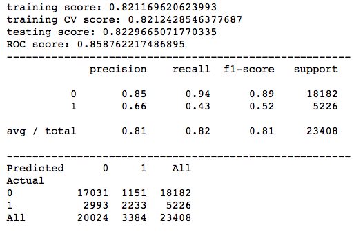
Model performance will be judged based on 3 key criterias:-
- Confusion matrix results (TN, FP, FN, TP)
- Accuracy scores (training, cross validation, testing, AUC ROC)
- Precision and recall scores of the minority class
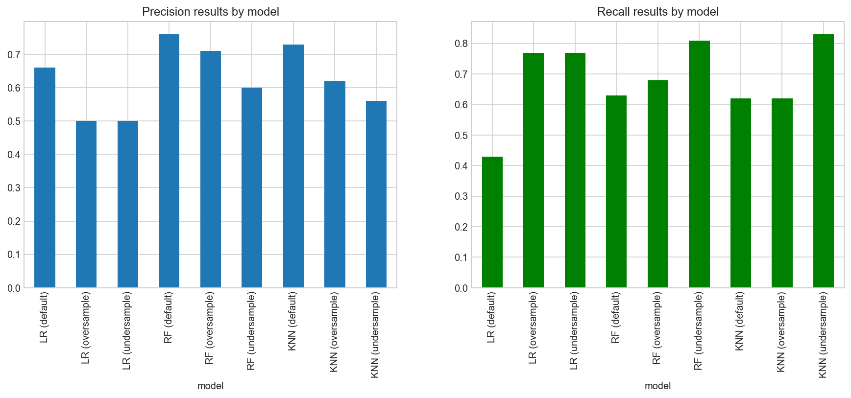
From the precision and recall graphs above, we can see an inverse correlation between them. Models that had a high precision result like Random Forest (default) and KNN (default) did not perform well in recall, while models with high recall results like KNN (undersample) and Random Forest (undersample) had a lower precision result.
Another interesting point to note is that default models achieved higher precision scores while models with undersampling had higher recall scores.
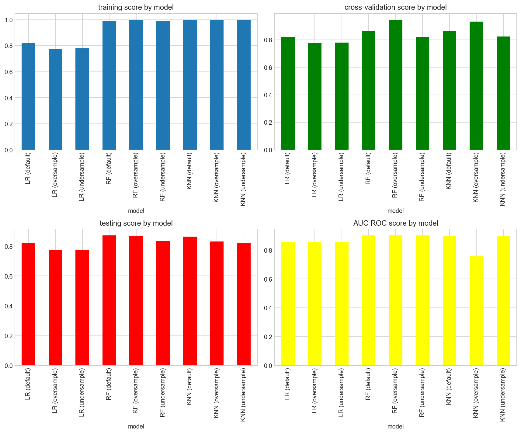
In terms of accuracy scores, our models will need to achieve an accuracy score that is higher than the baseline of 0.77408. From the results, all 9 models were able to exceed the baseline. The Logistic Regression models in general had the lowest scores, while the Random Forest models had the best.
When comparing the 4 accuracy graphs,the random forest (oversample) model was consistently able to achieve one of the highest scores across all 4.
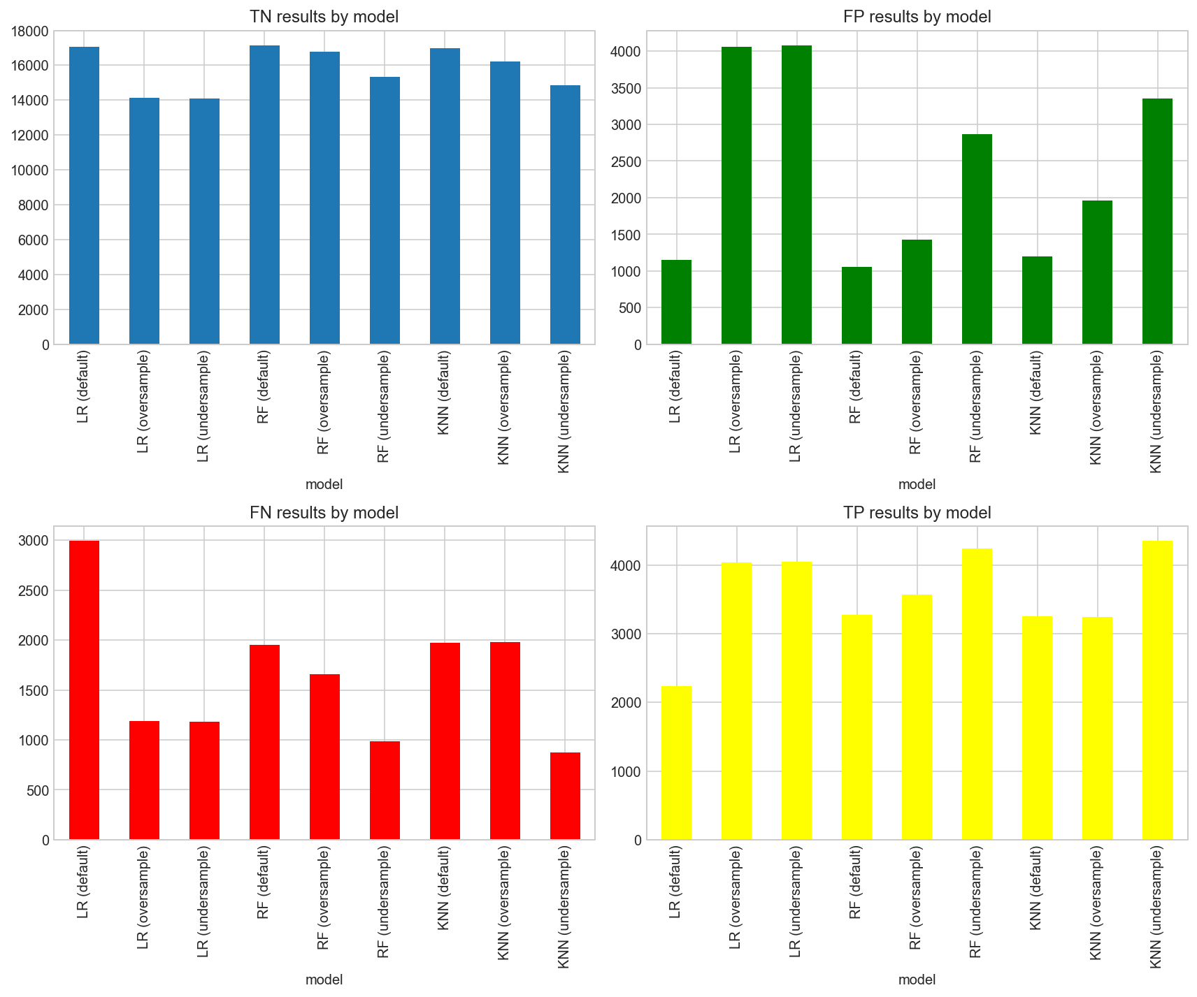
Looking at the confusion matrix results, the KNN (undersample) and Random Forest (Undersample) models had the highest number of correct predictions for the minority class (TP), while the Random Forest (default) and Logistic Regression (default) models had the most number of majority class predictions (TN).
In terms of wrong predictions, Logistic Regression (oversample and undersample) has the most Type I errors (FP) and Logistic Regression (default) the highest number of Type II errors (FN). This means that Logistic Regression models are unable to accurately classify the minority class and would be unsuitable algorithm to achieve our goal.
When comparing the Random Forest and KNN models, the undersampling models had the most False Positive (FP) errors and the lowest False Negative (FN) rates . On the other hand, while default and oversampling models may have a lower FP rate, their FN rate is higher.
3.5 - Model Selection
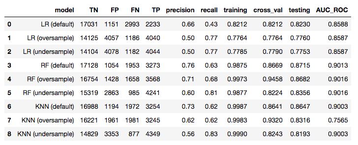
Since our goal is to predict the highest number of win opportunities, a model with high recall is desired. Being able to identify these accurately will mean more revenue for the business. Based on this, the K-Nearest Neighbors (undersample) model was able to achieve the highest recall score of 0.83, the highest True Positive (TP) rate of 4349, and lowest False Negative (FN) rate of 877. While its Type II error (FP) is one of the highest out of all the models, it is more acceptable to wrongly predict a loss opportunity than an inaccurate prediction of a won opportunity. Therefore, this model would be most suitable to achieve our goal of predicting the opportunity outcome.
Conclusion
After constructing our predictive models and analysing the results, we can conclude that the goals that were originally set have been achieved. The Ridge Regression model is suitable to predict the value of sales opportunities, and the K-Nearest Neighbors (undersample) model can be used to predict the outcome. Overall, this project demonstrates the usefulness of machine learning in creating business insights.
To view the full code, please check out the links below:
Part 1 Pre-Processing
Part 2 Predict Opportunity Amount
Part 3 Predict Opportunity Outcome